Hockey

Trying to Escape Mediocrity, The State of the Blues

 Ryan McKenzie

March 21st, 2025

The St. Louis Blues in the 2010’s were one of the more successful franchises in the NHL. The team’s winning percentage in the decade was 56.4%, which was the 3rd best in the league throughout this time period. These regular season successes propelled the Blues into consistently making the playoffs. Between the years 2011 through 2020, the Blues only missed the playoffs one time. They won the central division 3 times during this span, and in 2019 the franchise achieved hockey’s ultimate goal by winning its first-ever Stanley Cup. Since 2020, however, the Blues have made many missteps leading to a steady decline in the team’s performance.

Fast forward to after the unique 2020-2021 NHL season which was an anomaly for all teams. There were no out of division games, and the divisions were rearranged due Covid restrictions in Canada. Even so, the Blues appeared to be on a downward trajectory after losing in the 1st round of the playoffs in back-to-back seasons and only winning two total playoff games in those two series. Even after a bounce-back 2021-2022 campaign, when the Blues garnered a 109-point regular season culminating in a first-round takedown of the Minnesota Wild in 6 games, it is now clear that the Blues were at the end of an era. A lot of the team’s best players from 2019 were getting older and could not carry a team like they did in the past. 

Throughout the seasons following the 2019 Stanley Cup victory, the championship core roster was starting to break apart, either due to age or free agency. And, unfortunately, the Blues’ management did not adequately adjust in order to keep their roster playoff caliber. The first mistake the team made was trading for and immediately extending the contract of Justin Faulk in the summer of 2019. Faulk was a three-time all-star in Carolina and was talented in creating offense, but was an odd fit for the Blues as their defense was its primary strength. While Justin Faulk has had a couple of decent seasons in St. Louis, he has also had some rough seasons. Add to that inconsistent record, the fact that he is 32 years old now and has two more seasons left on his 6.5-million-dollar contract, it is unlikely things will improve. Although the Faulk move was puzzling at the time, the most shocking decision the Blues made was not extending the contract for team captain and elite defenseman Alex Pietrangelo. Pietrangelo had been the heart and soul of the Blues’ blue line for 12 seasons and was the first player in Blues franchise history to lift the Stanley Cup. Nevertheless, General Manager Doug Armstrong decided to play hard ball with the team captain in contract negotiations, and it led to Pietrangelo signing with the Vegas Golden Knights in free agency. In the 2021 offseason, the Blues suffered another defensive loss when the Seattle expansion draft led to the Blues losing a productive young defenseman in Vince Dunn. In an attempt to strengthen the defensive core, the Blues then signed Bruins’s defenseman Torey Krug to a 7-year 45.5-million-dollar deal. However, Krug is a smaller offensive defenseman, which has proven a significant limitation on the ice. 

The era of mediocrity that began in the 2022-2023 and the 2023-2024 seasons led to the Blues missing the playoffs both seasons and finishing with the 10th and 16th draft positions in those years’ drafts. The team did not have enough star players and had a lack of young, high-end talent outside of forwards Robert Thomas and Jordan Kyrou. The Blues were frequently outshot in a majority of the games they played throughout these two seasons. The underlying numbers showed this reality as well. The Blues were bottom 5 in expected goals for at 5 on 5, which shows how their offense was not that good. During this time, the Blues frequently relied on the extremely good goaltending tandem of Jordan Binnington and Joel Hofer to bail them out in order to win games, but often it was not enough to make up for the subpar play by the team’s skaters.

This brings us to March of 2025, and the Blues remain suspended in the hockey purgatory of mediocrity in which the team is not good enough to make the playoffs but not bad enough to acquire a top pick in the NHL draft that might turn the franchise around. One silver lining, however, is that for the first time since the 2021-2022 season, that the Blues appear to have a cohesive team that is playing well together. Although the start this season seemed to be more of the same St. Louis. The Blues were hovering in the 9th to 12th position in the western conference with no potential to make any noise, they caught fire last month after the 4 Nations Face-Off tournament break. They are now 10-2-2 since the break and it’s not just the results of the games that are encouraging, the way the Blues are playing is eye opening. They are controlling games now, with an offense that has come alive. The team is exerting much more control in the offensive zone. And the Blues have been extremely lethal on the rush. They are creating consistent scoring opportunities. They put up five goals against the Wild and Capitals during this run and have put up seven goals against the Kraken and Ducks during the last month. Looking ahead, the Blues have the easiest remaining strength of schedule and are currently one point ahead of Vancouver, and two points ahead of Calgary for the final wild card spot in the Western Conference. But the race is still a tossup because the blues have played more games than Vancouver, Calgary and Utah. If the Blues continue to play as they have this late in the season, those final games should be wins.

This abrupt turnaround did not happen overnight. No Matter how the rest of this season plays out, it is clear that Head Coach Jim Montgomery has been making all the right moves since he was promoted to the position last year. Montgomery, a former Blues assistant coach who had been recently let go by the Bruins, was tapped after the Blues fired its head coach Drew Bannister 22 games into the season, in mid-November. Montgomery brought a winning track record during his time in Dallas and in Boston, where he led the Bruins to the greatest regular season in NHL history. And so far, he has been just as good as advertised in St. Louis, with the team’s winning record gaining steam. Most of St. Louis’ best players today are on the younger side and they have a couple highly touted prospects that could help out the team soon.

Other strategic moves that helped the Blue included giving offer sheets to Oilers’ forward Dylan Holloway and defenseman Phillip Borberg, after most of the unrestricted free agents had already been signed. The Oilers were cap strapped and decided not to match the contracts the Blues handed out. Both players were young, former first round picks for Edmonton who had not had a lot of opportunity for the contending Oilers and had not broken out yet. Broberg has been the speedy, big, mobile defensemen the Blues have been looking for and has proved to be a terrific signing, and Holloway is third on the team in points, with 56 points in 70 games as of this writing. The Blues needed more young offensive skill, and Holloway has definitely brought that to the team. He is fast and has a phenomenal one timer that has helped boost the Blues on the power play this year.

Then, on December 14, the Blues traded for Ducks defenseman Cam Fowler for a 2nd round pick in 2027 and a prospect. Fowler did not have great numbers in Anaheim to start the year so many questioned this move, but Fowler has turned it around and is averaging a little over 0.5 points a game for the Blues and has been playing lots of big minutes for the Blues (even more so now without the Blues’ best Colton Parayko sidelined for 6 weeks with injury at the moment). Finally, the Blues in January waived forward Brandon Saad who posted a team worst -14 plus minus and was not contributing towards the team’s offense like he had in previous seasons. Not only did the Blues waive Saad, both sides agreed to terminate the contract in order for Saad to sign somewhere else in the NHL somewhere instead of being demoted to the AHL. This contract termination was a mutual decision between the team and Saad. While Armstrong has made a lot of questionable decisions in recent years, this season he has seemed to pull the right levers at the right time.

Clearly, the future is looking much brighter for the St. Louis Blues, and if they continue to develop, this recent run could be a sign of things to come. There are going to be challenges for the Blues to become a consistent playoff contender, but for the first time in a couple of years, there is hope for this team to be a winning team that might lift the Stanley Cup again sometime in the future.

Researching NHL Postseason Skater Production Differentials Using Machine Learning

Michael Southwick

October 13th, 2024

Introduction 

One of the most common narratives in professional hockey surrounds the differences between the regular season and the playoffs. It is often discussed that the faster, more physical nature of postseason hockey plays as a different game than what is commonly seen during the regular season. Many theorize that certain skaters have the capacity to better adapt to this style of playoff hockey, taking on a new role compared to their regular season play. Research in this area could provide new insights to teams for acquiring undervalued skaters through the regular season who have increased potential to become playoff difference makers.  

This paper serves to accomplish three main primary goals: 

1. Research the tangible differences between regular and postseason hockey in the NHL that can help provide context towards the types of skaters that excel during the playoffs.  

2. Develop a model inputting playstyle-driven regular season variables that will predict the difference between any skater’s regular season and postseason production.  

3. Discuss model strengths & weaknesses and provide possible applications for this research. 

Data for this project is sourced from the NHL’s public API from seasons 2020-2024 and publicized NHL EDGE data. References to Expected Goals in this work are using a personal model created which is competitive with standard public xG models.  

1. Exploratory Data Analysis for Differential Trends 

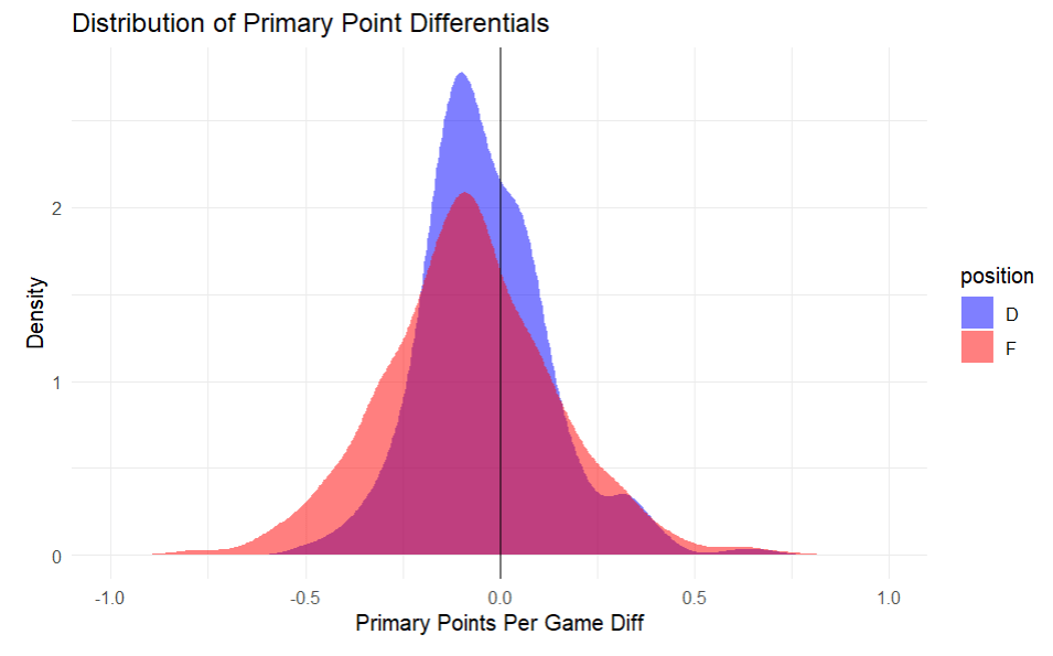
One of the first considerations in forecasting individual production differentials is to gauge how general production varies from the regular season to the postseason. The main figure that will be used to stand in for production are primary points (goals + primary assists) per game. The differential is a simple equation: postseason primary points per game – regular season primary points per game and is represented by P1DIF. The figure on the right highlights slight drop-offs as skaters enter the playoffs from their regular season production. For forwards, -.08 primary points per game, for defensemen -.04 primary points per game. 

One reason for this being that scoring is generally lower in postseason games compared to regular season games. For this next figure, games ended in OT were excluded, due to format differences for consistency. 

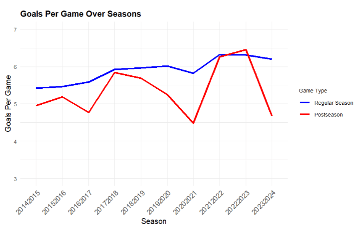
The figure above highlights the trends over time. Besides the 22/23 season, the regular season (blue) consistently shows higher per game scoring than the postseason (red).  

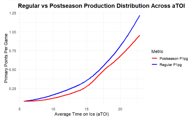
Depth being more valuable in the playoffs is evidenced by changes in lineup production distribution. The next figure to the right shows two smoothed curves, each showing the mean primary points per game at different average TOIs for forwards. Because scoring is higher in the regular season, the regular season curve remains above the postseason curve for the entire plot. The spread between the two curves minimizes in the range of 16-17.5 minutes per game and then widens as the curve trends above 20 minutes per game. Skaters playing in a more middle of the lineup role have a smaller drop in production into the postseason than both those playing significant forward minutes at 19+ per game and those playing less at around 12-15 per game. 

When it comes to on-ice differences, one of the aspects that becomes more important in the postseason is physicality. In the span from 2020-2024, the regular season averaged 45.2 hits per game. This is 28 less per game than the 73.2 hits per game averaged in the postseason.  

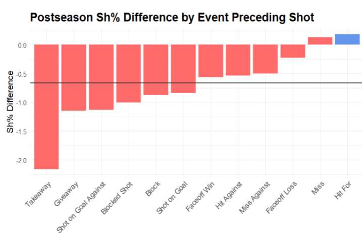
While this is notable, hits also become more effective in the postseason for generating goals. The figure on the right shows 12 events that can precede a shot attempt. The value on the y axis represents the mean difference in sh% for regular versus postseason shots. Hits for is one of two preceding event types that see a positive change in sh%. Across all 12 events, it is .72% less likely in the postseason that unblocked shot attempts convert to goals, however if following a hit for, it is .17% more likely a shot attempt is a goal. While the playoffs are more physical, this physicality is a greater catalyst to goal-scoring on a per shot basis. 

2a. Linear Approach 

The first approach is to model a set of independent variables against the P1DIF dependent variable through linear modeling. A couple of the input variables that ended up being relatively less important include xG_sa which represents the average quality of a skater’s shot attempt using xG. ONGp stands for on goal percentage, the percentage of shot attempts that were on goal. G_a is the ratio of goals to assists. EVp, PPp, & PKp are the % of ice time the player played at each strength. Five variables are also sourced from the NHL Edge data source: top_speed is the highest recorded player skating speed, burstspg is the # of 20+ MPH bursts a game, shot_speed is the top recorded shot speed, OZTp & DZTp are the percentages of time spent in the offensive and defensive zone respectively. Variables ending in _60 are counts per 60 minutes of ice time. 

The data for both the linear and non-linear approach used an 80/20 train/test split with each of the observations containing a player’s regular season variables with minimum four games played and a P1DIF dependent with minimum four playoff games. This linear regression is useful in revealing simpler, yet valuable insights that may be less apparent in the non-linear approach. Interaction terms and polynomials were introduced to the more significant predictors in this linear model, however success in increasing overall model effectiveness was limited.  

Two initial linear regression models were created, one for forwards and one for defensemen. After removing overwhelmingly insignificant variables, the output is shown in the figure to the right. Pts_60 being the most significant linear predictor with a p-value < .000 holds true with earlier findings about production distribution. This can be interpreted as, holding all else equal, for every increase in regular season of 1 point per 60, you would expect the player’s P1DIF to change by -.104. 

As shown with the figure on the left, the strength of variables is generally weaker for defensemen. Pts_60 is the strongest predictor for defensemen as well. These weaker relationships are likely a product of less emphasis being placed on the average defenseman compared to an average forward for generating goals, which makes it more difficult for discernable trends to exist year after year.  

2b. Non-Linear Approach 

The best model results were produced using non-linear models through the xGBoost framework. xGBoost, or extreme gradient boosting, is a machine learning model that takes advantage of decision trees and model correction to output non-linear trends in data. The xGBoost model also provides a high amount of hyperparameters that can be tuned for model effectiveness. A similar procedure is used for generating the non-linear model splitting the data between forwards and defensemen. The focus of the results here will be for the forward model due to what was shown in the linear forecasts. 

One of the key focuses in generating a proper machine learning model, is to avoid overfitting. Overfitting is the idea that the model will incorrectly fixate on specific examples present in the training data to build its trees. This is opposed to constructing trees that capture the overall trends in the data that should be equally present in the train and test partition. On the right, the graph shows the improvements to the RMSE, or root mean square error which is used for model evaluation throughout each iteration. Small deviations between the success of the test and train set occur around the 20^th iteration. A model of 35 rounds was selected where the test RMSE came out to .198 with a difference in RMSE between the train and test of .013 diminishing the possibility of overfitting having a major effect on model results. 

Many of the variables that showed low importance were removed from this model to reduce overfitting. For the importance matrix, the x-axis represents the % impact the variable has out of all variables for the output of this model.  

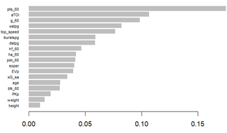
The figure to the left shows the importance matrix. Even in this non-linear model, regular season pts_60 is the most important variable in forecasting playoff production differential. This combined with aTOI and g_60 make up roughly 38% of model importance all roughly relating to the player’s role and production. After this comes ostpg (offensive zone starts per game) with dstpg (defensive zone starts per game) following closely. These zone starts are recorded when a player is substituted in for a faceoff in either the offensive or defensive zone. Exper stands in for the number of playoff games played before the current season and ends up having a relatively minor effect on model output, about 4%. Interestingly, two of the NHL EDGE data points make up about 13% of the importance in the model with both top_speed and burstspg placing highly. Then finally is a cluster of variables more closely related to physical play, with hf_60, ha_60, and pim_60. 

3. Model Evaluation & Potential Uses 

To put these RMSE values in context, it’s important to calculate a relative RMSE based on the range of P1DIF removing outliers. For forwards, there are 778 non-outlier observations resulting in a range from (-750, .600) yielding a rRMSE of 14.67% considered roughly standard for a good model. For the defenseman model there is an RMSE of .155 in an outlier-free range of (-.511, .451) resulting in an rRMSE of 16.11%, still solid, but not as effective as the forward model especially considering the defenseman model is poised for a greater risk of overfitting. 

To put some of these figures in comparison and illustrate some of the prediction difficulties, it’s interesting to look at same-player consistencies in P1DIF season over season. External factors play a role in making the differentials difficult to predict. These factors include the quantity of games played affecting the volatility of per game statistics in small samples, the quality of the opponents faced from playoffs to playoffs, differences in regular season and postseason deployment, among others. To test this, the 357 forwards in this span of 2020-2024 who had two consecutive seasons with enough games played were inputted using the previous season differential as a predictor for current season differential. The result is an RMSE of .345 or an rRMSE of 25.56% which yields distinctly less reliable results than the test data from the model built. This suggests that using the model built would be more effective in predicting the league’s playoff performers than simply looking at the previous season’s production differential.  

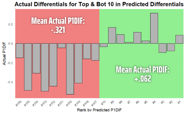
A last, more tangible way to get a sense of how the model forecasts best is to look towards the extremes of the predictions. Most important to note is that the following predictions only contain entries applied from the test data—they have never been seen by the model before, so a similar level of accuracy could be a reasonable expectation for future use. The chart on the right highlights the top and bottom 10 in terms of predicted differentials out of the 156 observations in the test data with the bar chart showing the actual differential. This yields promising results where, considering the mean P1DIF is -.096, the top 10 in predicted P1DIF are on average .75 standard deviations above the mean and the bottom 10 on average are 1.06 standard deviations below the mean. Examples of observations in the top 10 include 2021/22 Alex Iaffalo, 2020/21 Gabriel Landeskog, 2022/23 Trevor Moore, and 2022/23 Ondrej Palat. Examples in the bottom 10 include 2023/24 Mitch Marner, 2022/23 Jared McCann, 2020/21 Nikolaj Ehlers, and 2023/24 Nikita Kucherov. 

The best practical application of this model would assist teams focusing on playoff success through acquiring players who may be undervalued based on their regular season production but are slated to improve during the postseason.  

One specific example of this would be targeting players who may have very little playoff experience and as a result, uncertainty regarding how their playstyle would perform at the postseason game. Using the constructed model, you could run regular season results to see how similar players have performed historically. To demonstrate, I performed this exercise on the regular season performances from all 2023/24 regular season forwards and the output is shown in the chart to the right for the top 10. 

Considerations & Future Work 

To conclude this paper, I’d like to briefly recap the key points in each of the sections and discuss how this work could be improved in the future. 

1. When compared to the regular season, scoring is consistently lower in the playoffs. On average, all players are scoring less in the postseason, but this effect is least extreme for middle of the lineup players who absorb a larger role in production. Not only is the postseason significantly more physical, but hits are increasingly valuable for offense towards converting shot attempts to goals. 

2. Using an xGBoost model, there is greater accuracy and relevance in predicting forward production differentials compared to defensemen. The most important variables for this forecast are role-related stats including pts_60, aTOI, and g_60. These are followed by zone shift start statistics (offensive & defensive), skating related statistics (bursts per game, top skating speed), and physicality related statistics (pim_60, hf_60, ha_60). 

3. Despite the nature of this data being highly exposed to external factors and random noise, there is good evidence that supports the model’s effectiveness. The model is more accurate in predicting production differentials compared to using the previous season’s differential. At the extremes able to accurately split top and bottom performers by nearly 1 standard deviation in untrained datasets. 

For future improvement, the primary area of interest would be looking deeper into how separable the effects of deployment and quality of competition are between players who are highly adaptable for postseason hockey. The model as it stands can provide some real valuable overall insights, but this information would allow teams to better strategize and optimize the deployment of forwards and defensemen and how to search for players who may be over/under utilized in their systems leading to inefficient results. The model can be best used as a tool that can predict the players who are most likely to be beneficiaries of playoff hockey. This is especially true when there is a low sample of prior postseason data to reference, or a team is looking to acquire a potentially undervalued player to contribute to playoff success. 

Building a NHL Player Goal Projection Model

Nick Sofianakos

July 30th, 2022

How often does a hockey player score the same amount of goals as the season before? How well can you predict the number of goals a player scores in a given season based off of previous seasons? As a hockey enthusiast just getting into analytics, I attempted to create a XGBoost model for the first time. According to my model, you can predict the number of goals a player scores in a given season pretty accurately. Using Rstudio and the NHL API package, I was able to create a model that can accurately predict the number of goals a given player in the National Hockey League will score that season based off of the previous four seasons he played. Because XGBoost performs incredibly well on structured datasets when doing a predictive modeling problem,  I chose XGBoost as my model type despite the plethora of other models. In addition, the XGBoost model was going to give me the best accuracy due to its gradient boosting algorithm. Throughout the process of this project, I learned a lot about what it takes to successfully put together a meaningful Sports Analytics project that predicts future outcomes.

Overall there were 3 main steps throughout this entire process:

1)Data Collection

2)Data Cleaning/Feature Engineering

3)Modeling

Data Collection

The first step was retrieving the data to use for the XGBoost model. I did this through the NHL API package as it includes all the NHL information I need to create a dataframe that the XGBoost model can utilize successfully. The data from the NHL API that I loaded in included every game that every player had played in any professional hockey league including the minors and juniors. However, I did not need this much data. I only needed data for each player that included the year of that season, how many goals they scored, how many games they played, and their age. I needed to get it into a usable form that the XGboost could use to make accurate predictions. I first loaded hockey team rosters so that we could pull player ids in order to obtain individual player statistics. After using the player ids to pull player seasons from the API, I had the data I needed to move forward to the next step. Additionally, I only used players born in 1970 or later because this would give us a more accurate sample of players from the modern era. 

Data Cleaning/Feature Engineering

Now that I had a data frame that contained player data for every Hockey player that played some form of professional hockey, I filtered the data frame to include players who played in the National Hockey League. Next, I created a new variable called age which was found by subtracting a player’s birth year from the year of that specific season. I wanted to include the year of their season’s start, goals they scored each season, their age each season, and the number of games they played each season because my goal in this project is to build a simple model to give me experience with XGBoost while also creating something useful. Year of season start is included to mark the year that these events occurred while the other variables were more important to the building of the model. Age was important to include because it is important in recognizing a player’s goal trends. Lastly, the number of games played was included because the more games a player plays, the more goals they are likely to score. Following this, I was able to format the data to contain only the year of the season start, age, goals, and games for the most recent 4 year stretch of a player’s career. I chose the most recent four year stretch of their career because I believed it had the most predictive power in this situation.

Now, the data was finally ready to be passed into the XGBoost Model.

Modeling

I now had a data frame of every NHL player that played the game (1970 or later) and every 4 year span of their career in order to get training data from each part of a player’s career. It was finally time to create the XGBoost Model. I trained the model with 80% of the data and tested it using the other 20%. I trained the model using 22 iterations where each iteration improved the root mean squared error of the model. I decided on 22 iterations because any more would overfit the model and the test root mean squared error would start to increase. This is seen in a plot I made of root mean squared error vs iterations.

I applied the model to the data making predictions for both the train and the test set. Below are some results from the model including goals predicted as well as age,actual goals scored, and the root mean squared error. 

Overall, the root mean squared error of the predictions was 4.296, meaning that on average, the amount of predicted goals the XGBoost model predicted was about 4.296 from the actual amount of goals scored that season. 

Improving the XGBoost Model

With a root mean squared error of 4.296 the XGBoost model I created could certainly be improved. One way to decrease the root mean squared error of my model is to tune my model. Tuning is the process of maximizing a model’s performance without overfitting or creating too high of a variance. This is done by modifying the hyperparameters of the model. Some hyperparameters are the maximum depth of each tree, the learning rate and the number of trees we choose to utilize. However, tuning can actually increase the root mean squared error if we change the hyperparameter too much, which is called overfitting, as I mentioned above. A second and simple way to make the XGBoost model more accurate is to change what features I am passing into the model to predict goals. I decided to only pass in the goals a player scored. Maybe another statistic directly correlates to goals, which would allow the model to make more accurate predictions. 

Overall, I was very pleased with the results of the model as it was my first time building a XGBoost model. I will definitely improve on this model and tune it in the future. In addition, I look forward to using and learning more about XGBoost.